Understanding how the students in my course did on an exam includes visualizing the distribution of their scores. In the past I used two standard visualizations: a histogram of the letter grade and a scatter plot that showed the distribution (similar to a cumulative distribution function).
For example, consider a final exam that 49 students took. The exam was worth 35 points, so the thresholds for letter grades (90% = "A," etc.) were 21, 24.5, 28, 31.5. After converting each student's score to a letter grade, I generated a histogram of the letter grades (Figure 1), which clearly shows that the most common grade was a "B." To get more details, I also generated the full distribution of the exam scores (Figure 2).
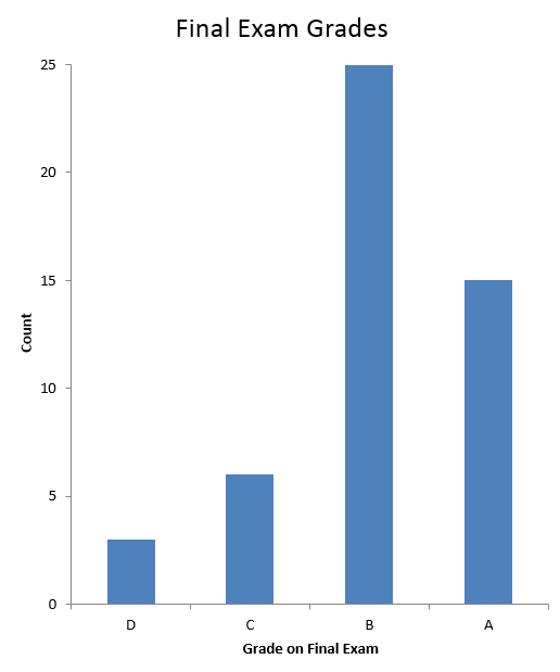 |
| Figure 1. The histogram. |
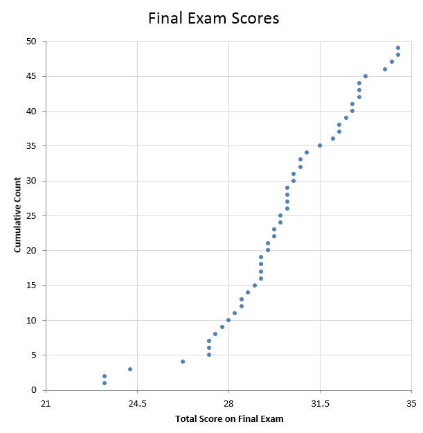 |
| Figure 2. The full distribution (each dot is one score). |
Although the vertical gridlines in the full distribution are on the thresholds for letter grades, there is a great deal of wasted space, and it is not obvious on this chart by itself which letter grade was most common. (In a larger data set, the vertical distance between points would have to shrink and could become too small to distinguish the markers.) To overcome this limitation, I changed the cumulative count to restart at each threshold, which yielded the chart (which I am calling a "distrogram") in Figure 3.
 |
| Figure 3. The distrogram. |
There are now four "curves," one for each letter grade, and each curve shows the distribution of scores in that letter grade. The height of each curve shows the total number of scores in that letter grade (as the histogram does). Thus the distrogram clearly shows that the most common grade was a "B." It also shows that the scores that correspond to "C" (between 24.5 and 28) were near the threshold for a "B" and that no one earned a perfect score (a 35). Thus, this distrogram provides the same information as the histogram plus additional information in a layout that is easier to navigate than the full distribution (the second chart). Because there are multiple curves, there is more vertical space between markers. Compared with the full distribution, however, the distrogram does require more operations to answer a distribution question such as "How many students earned at least 30 points on the exam?" because one would have to add the counts for multiple bins.
A distrogram should be useful for numerical data where the individual values and their grouping into categories (such as letter grades) based on these values are important. The key feature is that the simple bar in the histogram is replaced by a scatter plot showing the distribution of the values in that bin. Markers are needed to show the individual values; lines connecting the markers are not necessary; if they are used, they should be light so that the markers are easy to see. Horizontal and vertical gridlines should also be light if used.
To create a distrogram, define the thresholds for the bins and sort the values in ascending order. Determine the bin for each value. Add a cumulative count that starts at 1 and increases by 1 at each value (even if this value and the previous one are equal). Reset the cumulative count to 1 when the new value and the previous value are in different bins. Create a scatter plot, with the values on the horizontal axis and the cumulative count on the vertical axis